Gamma Distribution
This is the opposite of Poisson Distribution. In poisson, we measure how many rare events would happen in a fixed continuous interval.
In Gamma, we measure how much continuous interval would require for a fixed number of rare events to occur.
| Distribution | What is Fixed? | What is Random Variable | Question Asked |
|---|---|---|---|
| Poisson | Time () | Number of Events () | "In 1 hour, what is the probability I would get 5 calls?" |
| Gamma | Number of Events () | Time () | "To get 5 calls, what is the probability I have to wait 1 hour?" |
Since the random variable is the Continuous Interval, this is a Continuous Distribution.
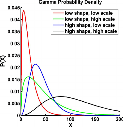
Gamma distribution is defined using two different parameterization methods.
- Shape-Rate parameterization ()
- Shape-Scale parameterization ()
This course will forward with the shape-scale parameterization
Interactive Graph - https://www.desmos.com/calculator/vk2tqrxpk5
Parameters & Key Properties:
- Shape (): Controls the profile and skewness.
- Scale (): Controls the horizontal scale/stretch along the -axis.
- Mean:
- Variance:
- Scaling Factor for Area to be 1 :
This is known as Gamma distribution since it uses the gamma function as the formula
Derivation of (Constant Factor)
We need the factor to keep the area always for given values Starting with generic Gamma based PDF,
\begin{align*} \int_{0}^{\infty} k x^{\alpha-1} e^{-\frac{x}{\beta}} \, dx &= 1 \\ k \int_{0}^{\infty} x^{\alpha-1} e^{-\frac{x}{\beta}} \, dx &= 1 \\ u = \frac{x}{\beta} \implies x = \beta u \implies dx = \beta \, du \\ \int_{0}^{\infty} (\beta u)^{\alpha-1} e^{-u} (\beta \, du) &= \int_{0}^{\infty} \beta^{\alpha-1} u^{\alpha-1} e^{-u} \beta \, du \\ &= \beta^{\alpha} \int_{0}^{\infty} u^{\alpha-1} e^{-u} \, du \\ &= \beta^{\alpha} \Gamma(\alpha) \\ \\ \end{align*}$$\begin{align*} k \cdot \beta^{\alpha} \Gamma(\alpha) &= 1 \ k &= \frac{1}{\Gamma(\alpha) \beta^{\alpha}} \end{align*}
## Shape Vs Scale 1. $\alpha$ - Changes shape/profile low $\alpha$ - skewed to left high $\alpha$ - more even like normal distribution Shape determines **how many** events we waiting for 2. $\beta$ - Changes horizontal stretch low $\beta$ - less stretch high $\beta$ - more stretch Scale determines **how many intervals** between 2 events | $\alpha$ change | $\beta$ change | | ------------------------------------------------------------------------------------------------------------------------------------- | ------------------------------------------------------------------------------------------------------------------------------------ | | ![[gamma-alpha.png]] | ![[gamma-beta.png]] | | Different profiling<br>$\alpha$= 1 - no left<br>2 - huge left skew<br>3 - less huge left skew<br>5 - more into even<br>10 - more even | Same profiling different stretch<br>$\beta$= 1 - tiny stretch<br>2 - a bit stretched<br>5 - more stretched<br>10 - further stretched | ## Properties - Gamma distribution has a additive property similar to [[Poisson Distribution]] Only when the **Scale** parameter is same.\text{If } X_1 \sim \text{Gamma}(\alpha_1, \beta) \quad \text{and} \quad X_2 \sim \text{Gamma}(\alpha_2, \beta)
\implies X_1 + X_2 \sim \text{Gamma}(\alpha_1 + \alpha_2, , \beta)