Poisson Distribution

This is a study of a total number of discrete events happening over a continuous interval unit (eg. Time, Space, area, volume)

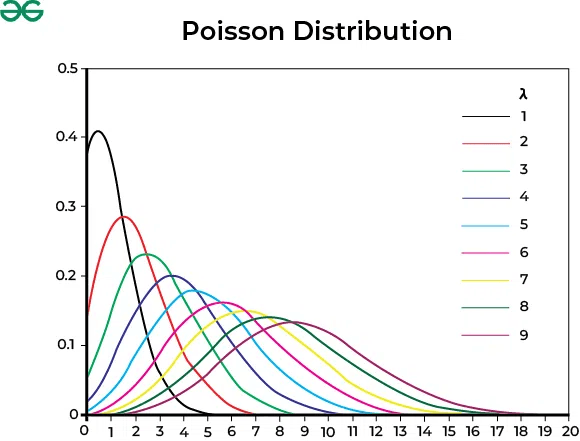
This distribution models the total number of times a rare event occur over a fixed interval. This is a discrete distribution since the random Variable is total number of events, which is a discrete.

Core Idea

We denote a Poisson random variable $X$ as:

Where:

• $\lambda$ (Lambda): The average rate (expected count) of events occurring in the given interval.
• $X$: The actual count of events observed ($X \in \{0, 1, 2, 3, \dots\}$).

3 Constraints

1. Constant Rate: Events occur at a known average rate $\lambda$ over a given interval.
2. Independence: The occurrence of one event does not affect the likelihood of another event occurring (e.g., one customer entering doesn't force another customer to enter).
3. Simultaneous Events Are Impossible: Two events cannot happen at the exact same instant (as the sub-intervals become infinitely small).

PMF

• $\lambda$ - Average Rate
• $k$ - Actual observed event count

Properties

Mean (Expected Value)

By definition, $\lambda$ is the average number of occurrences.

Variance

The spread increases directly with the average rate.

Scaling $\lambda$ for Different Windows

One of the best features of the Poisson distribution is how easily it scales. If the time window changes, you just scale $\lambda$ proportionally:

• If an emergency room gets $\lambda = 12$ patients per hour:
  • For a 30-minute window: $\lambda = 6$
  • For a 2-hour window: $\lambda = 24$

Relations to other distributions

1. Limiting case of [[Binomial Distribution]]

When the Binomial experiment has,

• Huge number of trials ($n \to \infty$)
• Small chance of success (i.e. Rare events, $p \to 0$)
• moderate expected value ($\lambda = n \cdot p$)

Rule of Thumb If $n \ge 20$ and $p \le 0.05$ (or $n \ge 100$ and $np \le 10$), the Poisson distribution provides an excellent, computationally cheap approximation of the Binomial distribution.

2. Poisson and Exponential (Two Sides of the Same Coin)

If events occur according to a Poisson process with rate $\lambda$:

• Poisson Distribution (Discrete): Counts HOW MANY events happen in a fixed time window.
• Exponential Distribution (Continuous): Measures HOW MUCH TIME passes between consecutive events.

Example: If a website gets an average of $\lambda = 10$ visits per minute (Poisson), the time you wait between visits follows an Exponential distribution with mean $\frac{1}{10} = 0.1$ minutes (6 seconds).

3. Poisson and Gamma / Erlang (Waiting for Multiple Events)

While the Exponential distribution models the waiting time for the 1st Poisson event, the Gamma distribution (specifically the Erlang distribution) models the total waiting time for the $k$-th Poisson event.

Notice how this parallels the discrete relationship between Geometric (waiting for 1st success) and Negative Binomial (waiting for $r$-th success)!

4. Poisson and Normal (The Central Limit Theorem)

As the average rate $\lambda$ becomes large (usually $\lambda > 20$), the Poisson distribution loses its right-skewed shape and becomes symmetrical. By the Central Limit Theorem, it can be approximated by a continuous Normal distribution:

(Note: Since you are approximating a discrete distribution with a continuous one, you apply a continuity correction factor of $\pm 0.5$.)

                  ┌───────────────────────────────┐
                  │ Discrete Trial Distributions  │
                  └───────────────┬───────────────┘
                                  │ (n -> ∞, p -> 0)
                                  ▼
                         ┌─────────────────┐
                         │ Poisson(λ = np) │
                         └────────┬────────┘
                                  │
       ┌──────────────────────────┼──────────────────────────┐
       │ (Time between events)    │ (Time until k-th event)  │ (λ -> ∞)
       ▼                          ▼                          ▼
┌──────────────┐           ┌──────────────┐           ┌──────────────┐
│ Exponential  │           │    Gamma     │           │    Normal    │
│ (Continuous) │           │ (Continuous) │           │ (Continuous) │
└──────────────┘           └──────────────┘           └──────────────┘

Additive Property of Poisson (Summing Poisson Variables)

If you add two independent Poisson random variables together, the total count is also a Poisson random variable! The rates simply add up:

If $X \sim \text{Poisson}(\lambda_1)$ and $Y \sim \text{Poisson}(\lambda_2)$, then:

Example: If Call Center A receives $\lambda_1 = 5$ calls/hour and Call Center B receives $\lambda_2 = 8$ calls/hour, the combined center receives $X + Y \sim \text{Poisson}(13)$ calls/hour.